Results and Validation
Time-Series Validation Strategy
To prevent any data leakage and simulate a realistic use case, we maintained a strict chronological split between training and final evaluation:
- Training Set (2012 → End of 2021): This dataset is used to train both the base model (AR + calendar) and the residual correction model based on weather variables.
- Final Test Set (2022 → 2024): This dataset remains completely isolated during development and is utilized only once for the final evaluation reported in this tutorial.
This approach ensures that the presented performance reflects a genuine ability to generalize over time. The split strictly respects the chronology of the data and reproduces the actual conditions of a real-world forecasting environment.
Additionally, using a simple linear model (LinearRegression) helps mitigate overfitting risks and facilitates the interpretation of the results.
Thanks to this two-stage architecture—a base AR + calendar model followed by a residual correction model built on thermal aggregates—we ultimately achieve a significant boost in predictive performance.
Over the 2022–2024 test period, the Mean Absolute Error (MAE) drops from approximately 26,300 MWh for the AR + calendar model to around 24,307 MWh once meteorological variables are integrated. This represents a reduction of about 1,993 MWh, or roughly a 7.6% improvement over the baseline error.
While this gain might seem modest in absolute terms, it is highly significant in the context of large-scale energy systems, where even minor forecasting improvements can yield substantial operational benefits.
Qualitative Model Behavior
An initial way to analyze the impact of the weather variables is to directly compare the predictions of the base model against those of the final model over a representative period.
The selected window covers February 2022, a winter period marked by several significant variations in electricity consumption linked to changing thermal conditions.
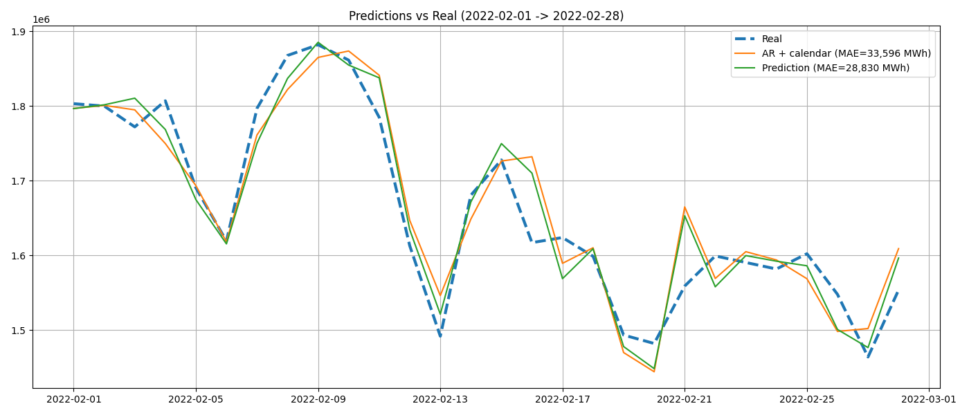
Figure 3 — Comparison of base model (AR + calendar) and final model predictions against actual consumption over a representative winter period (February 2022)
The AR + calendar model already reproduces the general dynamics of the series quite well, confirming the predictive value of autoregressive information and calendar-related variables. Most weekly patterns and major winter consumption peaks are captured correctly by this baseline model.
However, noticeable discrepancies remain during some periods of rapid demand variation, particularly around winter consumption peaks.
Adding meteorological variables helps correct part of these errors. The final model follows the observed series more closely on several sequences, especially during rapid thermal transitions observed throughout the month.
On this test window, the mean absolute error (MAE) decreases from approximately 33,600 MWh for the AR + calendar model to about 28,800 MWh after adding the meteorological correction, corresponding to a local improvement of roughly 14%.
More generally, this result is consistent with the central idea developed throughout this tutorial: thermal variables mainly provide complementary information that helps refine electricity demand forecasts when weather conditions have a strong influence on energy consumption.
Error Distribution
The improvement observed visually can be quantified by comparing the distribution of absolute errors over the same period.
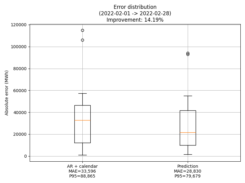
Figure 4 — Distribution of absolute errors for the base model and the final model (February 2022)
Analyzing the error distribution confirms the observations made on the prediction curves.
The median absolute error decreases noticeably after adding the weather variables, indicating that the corrected model improves not only a few isolated cases but also a significant share of routine forecasts over this winter period.
The effect is even more pronounced in the upper tail of the distribution. The 95th percentile of absolute errors drops from approximately 88,900 MWh to around 79,700 MWh, representing a reduction of nearly 10%. Consequently, the largest errors become both less frequent and less severe once the meteorological correction is introduced.
This improvement aligns with the role played by thermal variables: they provide valuable additional information primarily on days when weather conditions heavily influence electricity demand, particularly during the most severe winter snaps.
These results suggest that integrating thermal aggregates does more than just improve average forecasting accuracy. It also helps make the system more robust when facing the most challenging scenarios to predict, which happen to be the most critical from an operational perspective.