General introduction
Important
The source code for the scripts associated with this tutorial, along with the data required to run them, can be downloaded from GitHub. For details, please refer to the appendix 1.
Forecasting the discharge of large rivers plays an essential role in many areas: water resource management, dam operations, river navigation, hydropower generation, and flood forecasting. Having a reliable estimate of discharge for the coming days enables managers to make operational decisions, often under very short time constraints.
In this tutorial, we focus on the Mississippi River at St. Louis, Missouri. This choice is not arbitrary. Located immediately downstream of the confluence with the Missouri River, this gauge station is influenced by an immense watershed covering a large part of the central United States. The variations observed at St. Louis thus result from hydrological phenomena occurring sometimes several hundred kilometers upstream, making it an excellent case study for multivariate forecasting.
The data used come from the United States Geological Survey (USGS), which provides a vast set of hydrological measurements freely accessible via various APIs. Among the many available variables, two were of particular interest:
- discharge (or streamflow);
- gage height.
These two quantities are naturally strongly correlated: when the river level rises, its discharge also tends to increase. They thus describe two different aspects of the same physical phenomenon.
Nevertheless, we chose to build this tutorial using discharge data. The reason is largely practical: over the study period, the discharge time series are remarkably complete, whereas the gage height series have several gaps and interruptions. In order to have a regular time series with no missing values that can be directly used by machine learning models, discharge is therefore the best choice.
The goal of this tutorial is not to provide the most performant hydrological model possible, but rather to show how to build step by step a realistic, reproducible forecasting pipeline that is simple enough for each step to be understood and reused by the reader.
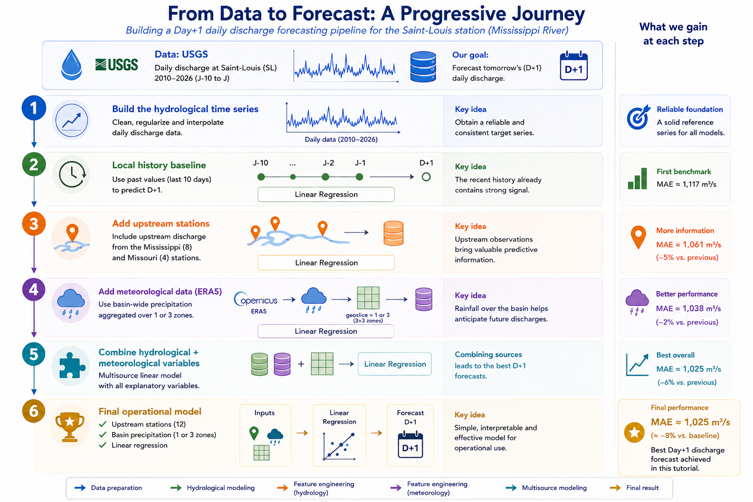
We will begin by building a clean hydrological time series, then compare several univariate approaches before progressively enriching the model by integrating upstream stations on the Mississippi and Missouri rivers. Finally, we will show how to leverage meteorological data from the ERA5 reanalysis to further improve the forecasts.
This progression illustrates a simple yet fundamental idea in time series analysis: the best performance often comes less from a complex algorithm than from a relevant representation of the data and careful engineering of the explanatory variables.
Tutorial Scope
This tutorial is above all educational in purpose. It aims to progressively build a complete hydrological forecasting pipeline using open data, while explaining the key steps of data preparation, feature engineering, and modeling.
Consequently, several analyses that would naturally belong to a comprehensive scientific study are intentionally left outside the scope of this tutorial. Their omission does not reflect a lack of interest but rather the educational objective of keeping the workflow simple and reproducible. We therefore do not investigate seasonal or hydrological-regime-dependent performance, nor do we specifically assess the prediction of peak discharges or flood events. Similarly, errors are not analyzed across different discharge ranges, exhaustive hyperparameter optimization is not pursued, and the tutorial remains limited to one-day-ahead forecasting with relatively simple models instead of exploring longer horizons or more sophisticated architectures such as recurrent neural networks or Transformers.