First experiments with univariate time series

In this section, we will build a first complete hydrological forecasting pipeline using a real-world time series from the USGS (United States Geological Survey) API. The goal is deliberately simple: predict the daily discharge of the Mississippi River at the St. Louis station with a one-day horizon, i.e., forecast tomorrow's discharge based on previous days.

This is a univariate problem: the model only has access to the historical discharge observed at this station. No meteorological data, no upstream stations, and no additional information are used at this stage. This approach allows us to understand what can already be achieved using only the internal dynamics of the time series.

The first step—building a clean, regular time series usable for forecasting—was completed in the previous section.

Recall that the script

station_download_daily.py

generated the file

07010000_daily_data.json

which corresponds to the St. Louis station and is the reference station we will use throughout the rest of the project.

This file contains a complete daily time series of 5,844 observations, with no missing values.

Note

Using the downloaded JSON file requires transforming it into a CSV file. This transformation is done using the script generate_series.py, which will be described in the next section (subsection "Final Harmonization").

Scripts used in this section

forecast_discharge_mono.py

Forecasting Objective

Using this time series, we will now compare several one-day-ahead (D+1) forecasting approaches:

a persistence baseline;
an XGBoost model;
a linear regression model using a sliding time window.

The script used for these experiments is forecast_discharge_mono.py.

Dataset splitting

An essential methodological point in forecasting is to strictly respect the temporal order of the data. Unlike a classic machine learning problem, observations cannot be randomly shuffled.

The script therefore splits the series into three distinct chronological sets.

Training dataset

Period:

2010-01-01 → 2020-12-31

This dataset contains 4,018 observations.

It is used to train the models.

Validation dataset

Period:

2021-01-01 → 2023-12-31

This dataset contains 1,095 observations.

It is used to compare models and adjust any hyperparameters.

Final test dataset

Period:

2024-01-01 → 2025-12-31

Ce datThis dataset contains 731 observations.

It is kept separate until the end and serves as a true test on the "future." It allows evaluation of the models' actual generalization ability.

This split is very important: no future information is used to predict the past. The pipeline thus avoids temporal leakage.

Persistence Baseline

The first model is deliberately trivial.

The persistence model simply assumes:

\[ Q_t \approx Q_{t-1} \]

In other words: "tomorrow will be identical to today."

This baseline is extremely important in hydrology. Large rivers have strong inertia, which often makes persistence surprisingly competitive.

Results obtained:

================================================
PERSISTENCE BASELINE
================================================

Validation metrics
MAE   : 8613.254
RMSE  : 14686.183
MAPE  : 4.752%
sMAPE : 4.798%

Test metrics
MAE   : 8308.082
RMSE  : 14737.902
MAPE  : 4.434%
sMAPE : 4.485%

The performance is already very good: the mean relative error remains below 5%.

This immediately indicates that the time series has a very strong temporal autocorrelation.

Notes on the Evaluation Metrics (Validation Set)

MAE (Mean Absolute Error / Erreur absolue moyenne) : measures the average absolute difference between the predictions and the actual values. Here, the model has an average error of 8,613 units, indicating that this metric is relatively robust to outliers.
RMSE (Root Mean Square Error) : similar to the MAE, but it penalizes large errors more heavily. Its higher value (14,686) suggests that a few predictions exhibit substantial deviations from the actual values.
MAPE (Mean Absolute Percentage Error) : expresses the prediction error as a percentage of the actual values. The model achieves an average relative error of approximately 4.75%. However, this metric can become unstable when the actual values are close to zero.
sMAPE (Symmetric Mean Absolute Percentage Error) : a variant of the MAPE that alleviates the issue of values close to zero and treats underestimation and overestimation more symmetrically. In this case, it confirms the model's excellent overall accuracy (4.80%).

XGBoost Model

The second model uses XGBoost, a modern gradient boosting algorithm very popular for tabular data.

Unlike the persistence model, this model receives several explanatory variables constructed from past observations:

lag_1
lag_2
lag_3
lag_7
lag_30

as well as moving averages:

rolling_mean_7
rolling_mean_30

The model then attempts to learn a nonlinear relationship between these variables and the next day's discharge.

Result:

==================================================
XGBOOST WITH TIME-SERIES WINDOWING
==================================================

Validation Metrics
MAE   : 7720.229
RMSE  : 13288.012
MAPE  : 4.505%
sMAPE : 4.498%

Test Metrics
MAE   : 7637.613
RMSE  : 12611.364
MAPE  : 4.220%
sMAPE : 4.231%

XGBoost clearly improves upon the persistence baseline. However, the gain remains relatively modest.

This suggests that the time series likely contains few complex nonlinearities at the one-day ahead horizon.

Linear Regression with Time Window

The third model is ultimately the most interesting.

The principle consists of using the discharge values from previous days as explanatory variables.

For example, using a 5-day window:

\[ Q_t = f( Q_{t-1}, Q_{t-2}, Q_{t-3}, Q_{t-4}, Q_{t-5} ) \]

In this case, the model used is a simple linear regression.

The script automatically constructs the time windows using the function:

build_window_dataset()

Each row of the generated dataset contains the discharge values from the previous 5 days as input features, and the discharge on the following day as the target.

Results obtained:

==================================================
LINEAR REGRESSION - WINDOW SIZE 5
==================================================

Validation Metrics
MAE   : 6898.727
RMSE  : 11414.617
MAPE  : 4.242%
sMAPE : 4.249%

Test Metrics
MAE   : 6457.529
RMSE  : 11303.852
MAPE  : 3.792%
sMAPE : 3.816%

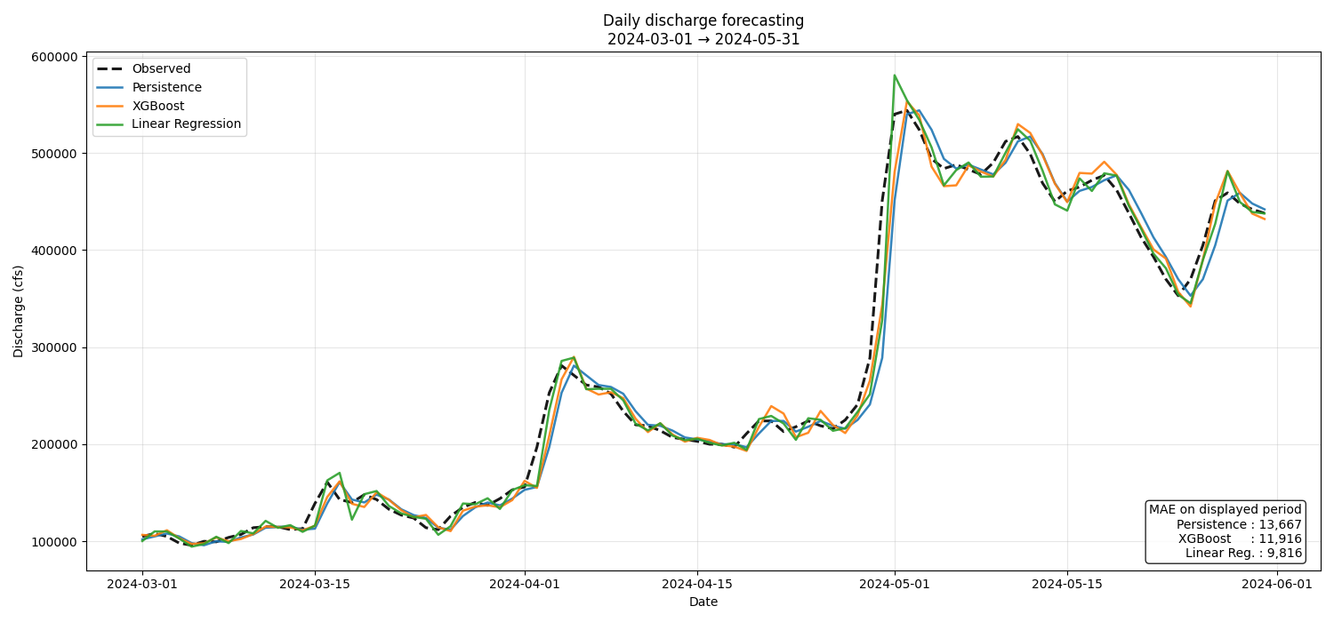
Figure 3 — Observed daily discharge of the Mississippi River at St. Louis and one-day ahead forecasts produced by three models (March–May 2024)

The result is very interesting.

Simple linear regression outperforms the persistence baseline, XGBoost, and several more complex variants tested previously but not included in the script (ARIMA, LightGBM).

We also tested more sophisticated regression models, such as Ridge, Lasso, and ElasticNet. We observed that they do not bring any significant improvement over this simple linear regression.

We will therefore keep a simple linear regression model incorporating a historical time window.

Interpretation of Results

These experiments show that the daily discharge of the Mississippi River at St. Louis is extremely predictable at a one-day horizon.

More specifically, the observed dynamics exhibit a high degree of autocorrelation and inertia, while remaining largely linear.

In other words, tomorrow's discharge strongly depends on the discharge values of previous days, following an almost affine relationship.

The fact that a simple linear regression outperforms more sophisticated nonlinear models is particularly interesting. This suggests that, in this univariate setting, complex models ultimately have little additional structure to exploit.

However, the improvement observed between persistence and linear regression shows that using multiple past days is clearly preferable to using a single time lag.

We also observe an interesting phenomenon: performance on the test dataset is systematically better than on the validation dataset. This behavior does not appear to come from temporal leakage, but rather from a difference in hydrological regime between the periods considered. The years 2024–2026 seem overall more regular and easier to forecast than the 2021–2023 period.

Finally, it should be remembered that this is only a first univariate prototype. The remainder of the tutorial shows how the model can be progressively enriched by adding information from upstream stations and by incorporating meteorological and spatial variables, thereby moving from a simple univariate approach to a genuinely multisource forecasting system.

In this richer multivariate context, models such as XGBoost or LightGBM could become significantly more competitive again.

×