Adding ERA5 Meteorological Features
In the previous sections, we progressively enriched our hydrological forecasting pipeline.
We first constructed a reference daily time series for the Mississippi River at St. Louis and then evaluated several univariate forecasting models. We subsequently incorporated upstream hydrological stations along the Mississippi and Missouri Rivers, which led to a substantial improvement in one-day-ahead (D+1) forecasting performance.
At this stage, the resulting pipeline is already fully operational.
This section—and the next one—may therefore be regarded as an optional extension of the tutorial.
In other words, you can stop here and still have a solid foundation for building a first hydrological forecasting model.
Why Go Further?
Because some of the information that influences river discharge is not always immediately reflected in the hydrological time series alone.
Streamflow observations describe the final outcome of several physical processes: precipitation, snow accumulation or snowmelt, infiltration, runoff, and finally propagation through the river network.
Part of this information will eventually be reflected in the upstream hydrological stations.
However, it may not appear there immediately.
Adding meteorological variables therefore makes it possible to introduce an earlier predictive signal: a period of intense rainfall or rapid snowmelt can be observed before its impact becomes visible in the streamflow records.
The objective of this section is to construct a meteorological dataset that is fully consistent with the hydrological time series prepared in the previous sections.
Scripts used in this section
create_era5_zoning.py
Choosing the Data Source
Several open data sources can be used to obtain daily meteorological data, among them NOAA GHCN Daily, the PRISM Climate Group datasets, and Copernicus ERA5.
For this tutorial, we selected:
ERA5 post-processed daily statistics on single levels
This dataset is available at:
https://cds.climate.copernicus.eu/datasets/derived-era5-single-levels-daily-statistics
This choice is motivated by several practical considerations.
ERA5 is particularly well suited to this application because it provides global coverage on a regular spatial grid, offers temporally homogeneous time series, and includes a large variety of atmospheric variables.
These characteristics make it a particularly well-suited data source for a reproducible machine learning workflow.
What Are ERA5 Data?
ERA5 is a meteorological reanalysis product developed by the European Centre for Medium-Range Weather Forecasts (ECMWF) as part of the Copernicus program.
The term reanalysis deserves a brief explanation.
ERA5 is not simply a collection of raw observations.
Instead, it combines information from multiple sources, including meteorological stations, satellite observations, radiosondes, buoys, and physical models of the atmosphere.
These different sources are assimilated into a single system to reconstruct, a posteriori, the most physically consistent representation possible of the state of the atmosphere.
The result is a dataset that is homogeneous both spatially and temporally.
For a forecasting project, these characteristics offer several practical advantages: the data contain very few gaps, remain consistent from one grid cell to another, and provide continuous coverage over long periods. This stability is particularly valuable when training and comparing models across multiple consecutive years.
The data are provided on a relatively fine spatial grid:
0.25° × 0.25°
Each grid cell covers an area of roughly a few tens of kilometers.
Selected Variable
For this meteorological integration, we will use only a single variable:
total_precipitation
his variable represents the total amount of precipitation accumulated over a single day.
It includes rain, snow, and other forms of precipitation such as freezing rain, sleet, and hail.
It is naturally a relevant predictor: a significant precipitation event may lead to an increase in the observed streamflow several days later.
Downloading the Data
Copernicus provides a Python API that can be used to automate data downloads.
It is highly convenient for production workflows.
In this tutorial, however, we chose not to use it in order to keep the procedure simple and easily reproducible through the web interface. The data are therefore downloaded manually, one year at a time.
Two parameters require particular attention.
Daily statistic
We select Daily sum
Why? Because the chosen variable represents a quantity accumulated over the course of a day.
For precipitation, the daily sum is therefore the most natural statistic to use.
Geographical area
The selected bounding box is: 49°N, -109°W, 37°S, -89°W
This area approximately covers the portion of the Mississippi River basin located upstream of St. Louis.
The goal is not to delineate the watershed exactly, but rather to define a sufficiently large region that encompasses the areas likely to influence the observed streamflow.
Corresponding API Request
Once the parameters have been selected in the interface, Copernicus automatically displays the equivalent Python request.
For example:
import cdsapi

dataset = "derived-era5-single-levels-daily-statistics"

request = {
    "product_type": "reanalysis",
    "variable": ["total_precipitation"],
    "year": "2010",
    "daily_statistic": "daily_sum",
    "time_zone": "utc+00:00",
    "frequency": "1_hourly",
    "area": [49, -109, 37, -89],
}

client = cdsapi.Client()

client.retrieve(dataset, request).download()
We then repeat this procedure for the total_precipitation variable, year by year, over the entire period from 2010 to 2025.
This results in a total of 16 NetCDF files.
The NetCDF Format
The files are downloaded in NetCDF (.nc) format.
NetCDF (Network Common Data Form) is a widely used format in climatology and atmospheric sciences.
It makes it possible to store multiple variables within a single file on a regular geographic grid while preserving their temporal dimension and the associated scientific metadata.
In practice, a NetCDF file directly contains the dates, the geographic coordinates of each grid point, and the corresponding meteorological values.
This format is particularly well suited to large datasets, as it facilitates the storage, exchange, and processing of complex spatiotemporal time series.
Constructing CSV Files
Why Aggregate the Data?
ERA5 files contain one precipitation value for each grid point and for each day.
Within our geographical area, this grid consists of 3,969 points.
In other words, if we were to use the raw data directly, a single day would be represented by 3,969 variables:
Day D

point_1
point_2
point_3
...
point_3969
With a 10-day temporal window, for example, the model would then receive nearly:
3969 × 10 ≈ 40 000
meteorological variables.
For a tutorial —and especially for a linear model— such a representation is unnecessarily complex. It greatly increases the computational cost and the risk of overfitting, while also making the experiments more difficult to interpret.
The Adopted Approach
Our objective is not to reproduce local meteorological conditions at high spatial resolution, but rather to provide the model with a synthetic indicator of the state of the river basin.
For a given region, we therefore compute the spatial average of precipitation over all grid points belonging to that region.
For example, if a region contains 441 grid points, the 441 daily values are replaced by a single one:
where (N) is the number of grid points in the region.
This average provides a simple summary of the overall precipitation level across that portion of the river basin.
Geographical Partitioning
We do not modify the temporal resolution: each row of the CSV file still corresponds to one day.
However, we simplify the spatial resolution.
Case z = 1
The entire study area is treated as a single region.
+-----------------------+
|                       |
|         basin         |
|                       |
+-----------------------+
The 3,969 daily values are replaced by a single spatial average:
date,tp
2010-01-01,...
2010-01-02,...
...
The resulting file therefore contains only one meteorological variable.
Case z = 3
The study area is divided into nine rectangles:
+-----+-----+-----+
|0,0  |0,1  |0,2  |
+-----+-----+-----+
|1,0  |1,1  |1,2  |
+-----+-----+-----+
|2,0  |2,1  |2,2  |
+-----+-----+-----+
Each rectangle is summarized by its daily spatial average.
The resulting file then contains:
date,
tp_0_0,tp_0_1,tp_0_2,
tp_1_0,tp_1_1,tp_1_2,
tp_2_0,tp_2_1,tp_2_2
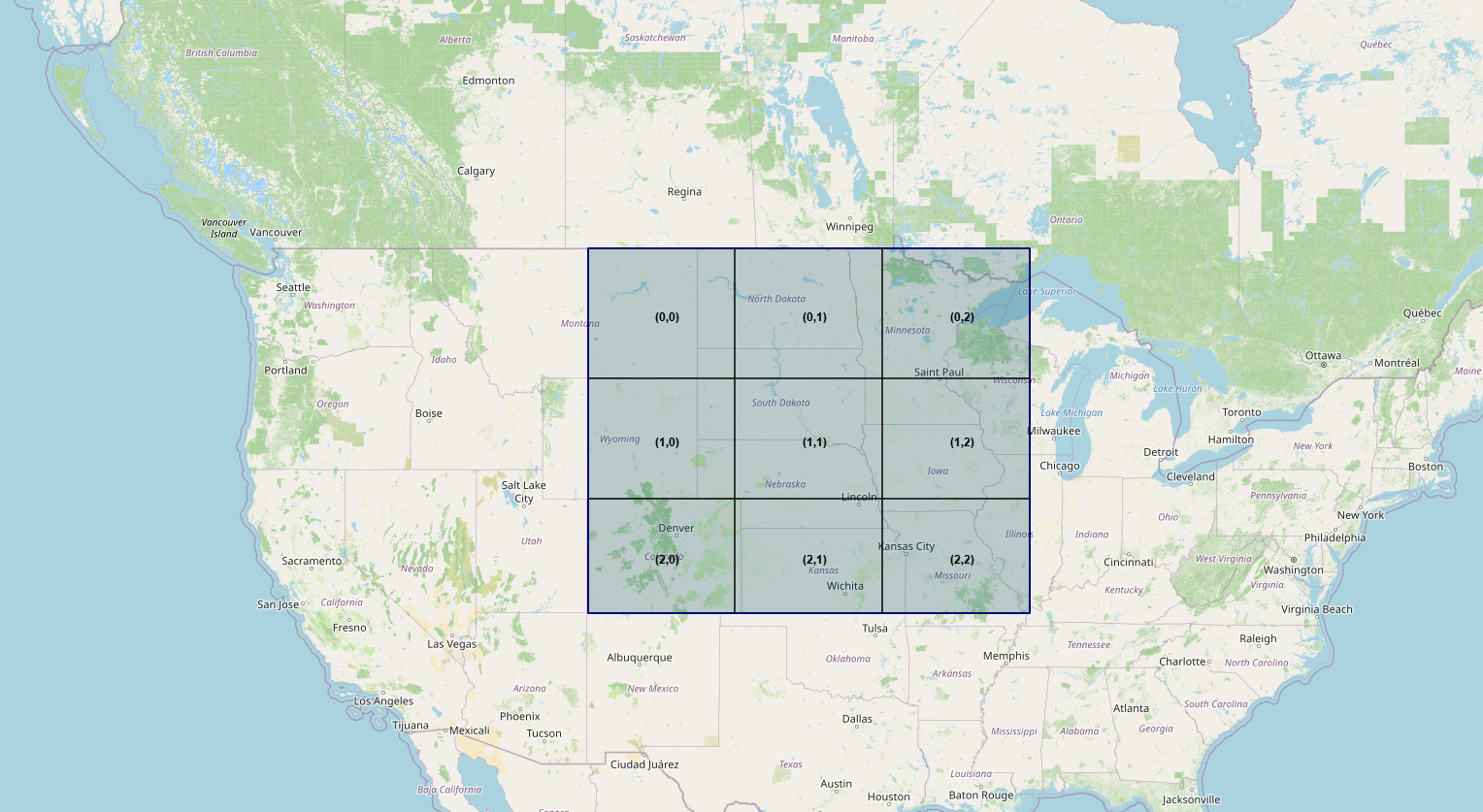
Figure 5.1 — Grid of the 9 total_precipitation variables
Each day is therefore represented by 9 variables instead of 3,969.
Generating the CSV Files
Once the NetCDF files have been downloaded, the data must be organized into a format that is easy to query.
The original ERA5 fields contain thousands of grid points. Within our study area, this corresponds to 3,969 values per day. If these data were used directly with a 10-day temporal window, the model would receive nearly 40,000 meteorological variables for a single prediction. Such a representation is unnecessarily complex for this tutorial and increases the risk of overfitting. We therefore construct a much more compact representation.
To accomplish this, we will use the script create_era5_zoning.py.
This script generates aggregated ERA5 time series for our hydrological forecasting experiments.
For each zoning level (z = 1, ..., 6), the study domain is divided into (z \times z) rectangular regions:
z=1  -> 1 region
z=2  -> 4 regions
z=3  -> 9 regions
...
z=6  -> 36 regions
For each region and each day, the spatial average is computed for the total_precipitation (tp) variable.
In this tutorial, we focus on only two zoning levels: 1 and 3. These levels are specified in the ZONING_LEVELS constant.
The script automatically generates two CSV files:
- era5_z1.csv corresponding to a single region
- era5_z3.csv corresponding to 3 * 3 = 9 regions.
Structure of the Generated Files
Column Naming Convention
For z = 1:
date,tp
For z>1
date,
tp_0_0,tp_0_1,...,tp_(z-1)_(z-1),
The first index corresponds to the relative latitude (0 = the northernmost region), while the second corresponds to the relative longitude (0 = the westernmost region).
Each column covers the period 2010-01-01 → 2025-12-31, corresponding to 5,844 values. We therefore obtain a meteorological dataset that is fully consistent with the hydrological time series prepared in the previous sections: the time span is identical, the temporal resolution remains daily, and the entire upstream basin benefits from continuous spatial coverage.
Why This Compromise?
This aggregation strategy represents a compromise between two extreme situations:
- using a single average over the entire basin (
z = 1), which loses much of the spatial information; - using all 3,969 ERA5 grid points, which results in an extremely large number of variables.
Dividing the study area into a small number of regions preserves part of the spatial structure of the precipitation field while keeping the number of variables at a reasonable level for the machine learning models considered in this tutorial.
In the remainder of the pipeline, this organization greatly simplifies data processing and makes the experiments more computationally efficient.
Practical Note
The download phase described above is the most time-consuming part of this section.
Manually retrieving the sixteen NetCDF files and verifying their consistency requires a significant amount of time.
If your primary goal is to experiment with the forecasting models as quickly as possible, we therefore recommend using the pre-generated CSV files directly.
Conclusion
This section is more closely related to data mining than to modeling itself. However, thanks to it, our forecasting pipeline no longer relies solely on hydrological observations.
We now have a second set of variables describing the meteorological conditions across the entire upstream basin. In the context of this tutorial, we have limited ourselves to a single variable: total_precipitation.
These data are not intended to replace the streamflow time series; rather, they are meant to complement them by providing an additional predictive signal related to precipitation.
In the next section, we will use the CSV files generated by the create_era5_zoning.py script to incorporate the selected ERA5 data into the forecasting pipeline and evaluate their actual contribution to forecasting performance.